Speculative Decoding Looks Slower? Check Tokens, Chunks and Load

If speculative decoding looks slower, first check what the timer counts. A streamed chunk can contain several tokens. Longer gaps between chunks do not necessarily mean more time per token. If the same completed workload really takes longer, compare the cost of proposing and verifying tokens with the number ultimately emitted, then repeat the comparison at the load your service actually handles.

This guide gives a measurement worksheet for that decision. The examples below are fictional arithmetic, not benchmarks. The vLLM references are rolling documentation checked on November 5, 2026; pin the server and benchmark versions before relying on their current fields or behavior.

Did generation slow down, or did tokens arrive in larger chunks?

The current vLLM benchmark guide distinguishes three client-side measurements:

• TTFT: request sent to first streamed output received.
• ITL: gaps between consecutive streamed outputs. With speculation, an output can contain multiple tokens.
• TPOT: each request’s time after the first output, divided by its total output-token count minus one, then aggregated across requests.

Use the actual measurement points, not just a chart labeled “latency.” A server’s internal timing and a client’s elapsed time need not cover the same work.

Consider two fictional responses containing six output tokens. Times below are milliseconds after sending the request; each number in parentheses is the token count in that chunk.

• Baseline: 100(1), 120(1), 140(1), 160(1), 180(1), 200(1). Mean chunk gap: 20 ms. TPOT: (200 − 100) / 5 = 20 ms/token.
• Speculation: 100(1), 135(3), 170(2). Mean chunk gap: 35 ms. TPOT: (170 − 100) / 5 = 14 ms/token.

In this invented trace, mean ITL worsens from 20 to 35 ms while completion improves from 200 to 170 ms. Both measurements are correct. One counts gaps between deliveries; the other spreads decode time over output tokens. Neither says whether the text is useful. A UI sensitive to pauses may still prefer smoother arrivals, so keep a chunk-gap objective if it matters.

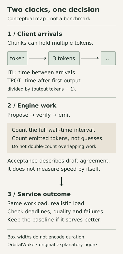
Read the arrival clock and the engine-work clock separately. This is a conceptual measurement map, not a measured timeline; box sizes do not represent duration.

Why can high acceptance still produce a real slowdown?

A draft proposes tokens; the target checks them. The original speculative decoding paper, Algorithm 1 and Section 3, analyzes how accepted drafts reduce serial target calls while adding draft work. Its wall-time result assumes sufficient parallel compute for verification and sufficiently long generations. Fewer target calls are therefore not a universal wall-clock speedup.

For an observed decode interval, a useful accounting check is:

Amortized decode time = total elapsed decode time / total tokens emitted during that interval.

Use disjoint interval boundaries and actual output tokens, not the number of proposals. If profiling draft, verification and other work separately, do not add overlapping GPU/CPU durations as though they were serial. For pipelined or batched engines, wall time and component work answer different questions.

A second fictional example: ordinary decoding takes 10 ms/token. One speculative cycle emits four tokens, including any correction or bonus token. If that entire cycle takes 30 ms, it costs 7.5 ms/token; if it takes 45 ms, it costs 11.25 ms/token. The emitted count is unchanged, but the first case wins and the second loses. This is break-even arithmetic, not a prediction for any model or device.

The current acceptance-metrics reference defines draft acceptance rate using accepted draft tokens divided by proposed draft tokens. That is different from emitted tokens per verification step: bonus tokens are excluded from the accepted-draft count. The per-request interface is experimental, defaults to disabled and reports only single-sequence requests. Confirm availability in your pinned version; a missing metric is not zero acceptance.

Why does the improvement disappear when more users arrive?

A quiet, memory-bound deployment can have spare compute for verification. Under heavier load, the extra work can compete with other requests. The vLLM team’s October 2024 performance analysis reported both improvements and regressions as workload and request rate changed. Those historical measurements are not current hardware guarantees.

Current dynamic speculative decoding documentation describes changing proposal length by concurrency range, including zero draft tokens in a configured range. That supplies a control to evaluate, not proof that one threshold fits every deployment. The proposed draft length, effective batch, model, sampling settings and available memory all belong in the comparison.

Do not choose a configuration from a single idle request if the goal is a multi-user service. A lower average decode time is insufficient when the fraction of requests meeting the service deadline falls. Conversely, total server tokens per second does not describe the experience of one interactive user.

What should an on/off comparison keep fixed?

Use a small workload matrix rather than one favorite prompt. The following is our proposed review procedure, not an experiment we ran:

1. Freeze the target configuration. Record model and tokenizer revisions, quantization, engine/build, hardware placement, context limit, sampling and stop rules. Record the drafter and proposal policy separately.
2. Choose the decision first. An interactive service might require both an acceptable first-output delay and an acceptable completion deadline. A batch job may care about completed, quality-accepted items per unit time. Set the limits before reading the results.
3. Cover the intended inputs. Separate short and long prompts, short and long outputs, and the task types actually served. Report actual output lengths and unsuccessful requests; a shorter or failed answer is not a speedup.
4. Compare quiet and representative load. Keep the arrival pattern and concurrency cap explicit. Alternate repeated on/off runs after comparable warmup. Do not silently give one configuration cached prefixes and the other a cold workload.
5. Keep a result row for each condition. Record completed-request count, output tokens, client TTFT/TPOT/chunk gaps, completion latency, throughput, failures, memory pressure and acceptance counters. Preserve distributions and tail observations, not only means.

The benchmark guide’s cache warning explains why repeated prompts can inflate throughput. It also cautions that per-request timing collection adds CPU overhead. Use comparable instrumentation, then confirm the chosen configuration with the instrumentation intended for production. Avoid interpreting a diagnostic run as an uninstrumented performance result.

If the draft pushes the deployment into memory pressure, address that separately using the inference-memory ledger. If a response ends early, check completion state and output limits before comparing its speed.

Does “lossless” mean identical text on every run?

No. The standard rejection-sampling algorithm is designed to preserve the target’s sampling distribution under its assumptions. That is not a promise that two sampled runs produce the same string. The vLLM guarantee section also notes floating-point and batch-related differences; it explicitly excludes its lossy FLy verification from the distribution-preserving guarantee.

Record which verification method you actually use. Keep output-validity and task-quality checks in the acceptance decision, rather than treating a technique’s name as a certificate. A different sampled sentence alone does not establish a defect; a systematic quality change needs investigation under controlled conditions.

Retain speculation only for the workloads where it meets the preselected user-visible objective without unacceptable quality, capacity or reliability regressions. Keep the no-speculation baseline as a real option. The useful conclusion is not “speculation is fast” or “speculation is broken,” but which configuration helps which workload, under which measurement boundary.